Erich Focht
This post describes some bits of the tuning activity which lifted the
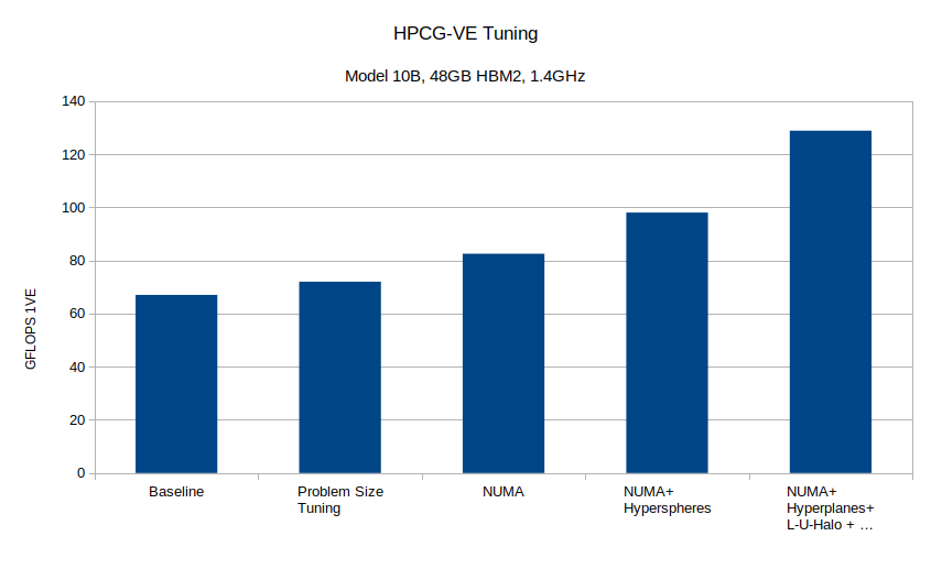
VE HPCG performance from ~67 GFLOPS to 125.5 128.8 GFLOPS on a
VE10B and nearly doubled the performance efficiency to 5.99%. Since
the first version of this post some more tunings of the setup and
optimization phases were done, raising the efficiency from the 5.83%
reported earlier. This revised version of the article also contains
new performance values for the 8 VE measurement on a NEC A300-8
system.
Introduction
During the past month I spent a bit of time on the HPCG benchmark, trying to tune it for the SX-Aurora vector engine (VE). The High Performance Conjugate Gradient benchmark complements the TOP500-defining High Performance Linpack (HPL) as it uses real-world applications data access patterns, inverting a sparse matrix with a conjugate gradient algorithm that uses a Gauss-Seidel smoothed multigrid preconditioner. Opposed to HPL, which is a compute bound benchmark with performance close to the peak performance of a supercomputer, HPCG is memory bound and achieves only small fractions of the peak performance. The current number 1 in the HPCG June 2019 list, Summit, reaches 1.5% performance efficiency.
SX-ACE Performance
NEC’s SX-ACE supercomputers are the entries into the HPCG list with the highest efficiency, ranging between 10.2 and 11.4%. Komatsu et al have described very nicely the tuning efforts for reaching this ground breaking efficiency eg. in this poster at SC15. The core takeaways from that effort are:
- the ELL matrix format, multicoloring and hyperplanes are well suited for the vector machine,
- the assignable data buffers (ADB) of the SX-ACE helps mitigate the SPMV/GS gather memory access,
- data rearrangements for contiguous access are important.
With 1 Byte per FLOP the SX-ACE is the machine with the highest relative memory bandwidth in the list, which explains its leading position.
SX-Aurora HPCG Baseline
The SX-Aurora vector engine shares the main ideas of the ISA with the SX-ACE, but is otherwise a completely different CPU and system. Two important differences are:
- the VE has approximately 0.5 Bytes per FLOP,
- there is no ADB, instead a Last Level Cache (LLC) which is shared among the 8 cores.
The baseline HPCG performance on the VE was described extensively by Prof. Kobayashi from Tohoku University in a presentation at the 28th WSSP workshop. On one VE of type 10B (1.4GHz) with 2.15TFLOPS double precision peak performance and 1.22TB/s memory bandwidth the HPCG benchmark reached 67 GFLOP and 3.1% efficiency.
The level of tuning of this baseline HPCG version is close to the SX-ACE version. It uses similar techniques for optimization, again the ELLPACK matrix format and hyperplanes equivalent to classical level scheduling for vectorization. It has a highly optimized kernel for sparse matrix-vector multiplication and tuned setup functions of which some may or may not use reverse offloading (VHcall).
VE HPCG Tuning
Problem Size
As seen from the WSSP presentation, the problem size influences quite a bit the performance of a HPCG run. This is understandable because hyperplane sizes vary a lot and with them the vector lengths. At the same time the memory layout and access pattern in the SPMV gather, too. The VE 4-way skewed cache is complicatng the story significantly. It improves the port conflicts for the access to the LLC cache fragments (see article on en.wikichip.org but makes the invalidation pattern random and hardly predictable.
In my very incomplete scan f the parameter space I was looking for a configuration that is rather long in one direction, such that hyperplanes sizes would increase quickly and stay constant for a longer time. I found a maximum at delivering 72 GFLOPS on the baseline code at:
nx=56; ny=216; nz=376;
Many of the following experiments were done with this local grid size: 56 x 216 x 376.
NUMA
Profiling HPCG runs with ftrace have quickly shown that the core routines ComputeSYMGS and ComputeSPMV suffer under a rather low LLC cache hit rate in the range of 30-33% and port conflicts. NUMA support for VEs has been released in VEOS at the end of June 2019 (see forum post) and is actually addressing exactly these issues: the LLC cache fragments and the cores are split into 2 groups which behave like separate NUMA domains. This reduces cache and port conflicts. And indeed, the HPCG tests showed a boost of the performance in NUMA mode to 82.5 GFLOPS.
Multicoloring, Hyperplanes and Hyperspheres
The permutation of the rows into a proper order that allows the vectorized (i.e. data parallel) update of elements is essential for increasing the performance. The hyperplanes approach is rather simple but fast. Its “colors” are actually a numbering of the hyperplanes and are incremented continuously. Each hyperplane contains rows whose nonzero lower matrix elements depend on the previous hyperplane.
Multicoloring is different, it effectively merges all colors of hyperplanes which have the same kind of dependency. The result in 3D based matrices is a grid colored into only eight colors. This results into longer vectors for the Gauss-Seidel substitution and higher performance of ComputeSYMGS, but increases the number of iterations to convergence. At the same time the longer lists of same-color elements lead to stronger thrashing of the LLC cache, at least in the current implementation. The performance could be larger with blocking but the convergence penalty made me rule out this method.
A third approach to reordering the rows is what I call Hyperspheres Ordering. To my knowledge this hasn’t been tried before so maybe details will end up in a separate paper. The core idea is to start the numbering in the middle of the grid instead of one corner, then enumerate the grid nodes in order of their appearance on spheres concentric to the starting point and with growing radius. The level scheduling algorithm is applied to this new ordering, creating hyperspheres of same level/color. The elements on these hyperspheres can be handled in parallel like on hyperplanes. By using this ordering the number of rows per hypersphere (thus the vectorizable loop lengths) are significantly larger than on hyperplanes. Also halo elements are “hit” late, at a rather high “color”.
The hyperspheres approach paired with the classical Gauss-Seidel algorithm increases the performance to 98 GFLOPS.
Tunings and Algorithm
The rest was … tuning, tuning, tuning and a some linear algebra that resulted from very inspiring discussions with Christie Alappat from the University of Erlangen. Many thanks to Erlangen!
The code now supports three optimized matrix formats: (1) ELLPACK with separated diagonal, (2) two ELLPACK matrices, one for the lower (L) and one for the upper matrix (U), with separated diagonal but including the halo elements, and (3) two ELLPACK matrices for L and U plus a separate ELLPACK matrix for the halo part. It also supports three reorderings: (1) Hyperplane, (2) Hypersphere and (3) Multicoloring. Finally: it supports a classical Gauss-Seidel substitution as well as one which uses L and U matrices separately and takes advantage of the symmetry of the Gauss-Seidel sweep.
Unfortunately the Hyperspheres approach turned out to widen the U matrix in ELLPACK format thus adding more padding entries than beneficial for the performance. I will investigate whether other matrix formats could work better, but had to switch back to Hyperplane ordering.
The setup phase GenerateProblem() was further vectorized, the typical nested loop pattern was linearized. Many pieces of OptimizeProblem() were offloaded to the VH by VHcall. There is still potential for improvement because actually the same data is being transfered to the VH several times. The well tuned sparse matrix-vector product kernel was rewritten, further unrolled and now avoids some unnecessary operations. Removing unnecessary operations had in the end a significant contribution to the result. DotProduct as well as WAXPBY were unrolled manually to increase performance, although their share is not so significant compared to SPMV and SYMGS. SPMV now uses some internal blocking that slightly improves the gathered data reuse.
The result of HPCG running on one VE 10B, with a pure MPI approach (8 processes) is:
GFLOP/s Summary:
  Raw DDOT: 230.742
  Raw WAXPBY: 106.772
  Raw SpMV: 98.1001
  Raw MG: 143.969
  Raw Total: 134.7
  Total with convergence overhead: 134.7
  Total with convergence and optimization phase overhead: 128.834
...
__________ Final Summary __________:
  HPCG result is VALID with a GFLOP/s rating of: 128.834
      HPCG 2.4 Rating (for historical value) is: 130.253
This corresponds to 5.99% performance efficiency.
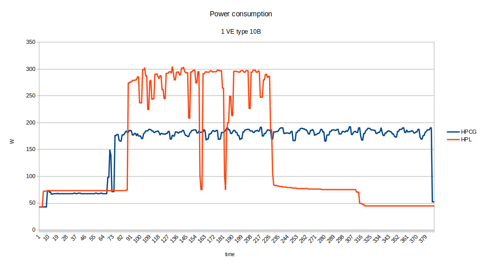
The power consumption during a HPCG run is noteworthy. I simply looped over a simple command like
vecmd info | egrep ^Current -A2 | grep -v Current | awk '{sum=sum+12*$5/1000}END{print sum}'
and stored the values of the current sensors on the VE card multiplied by 12V. The power reading is ignoring the vector host and should be compared to the TDP of the VE card: 300W. The figure below shows that HPCG consumes significantly less power than HPL on the VE:
First experiments show that a A300-8 with 8 VEs performs with approximately 870 GFLOPS with power consumption of the 8 VEs in the range of 1300W. While this is still above 5% efficiency, it shows that scalability might be an issue. I prepared the code for overlapping halo exchange and computation, but the lack of independent progress threads in the VE’s MPI are a problem that still needs to be tackled. Driving asynchronous MPI calls with MPI_Iprobe() works, but the benefit was limited.
NOTE November 12, 2019 With new measurements on A300-8 I reached in a long run
  HPCG result is VALID with a GFLOP/s rating of: 932.145
      HPCG 2.4 Rating (for historical value) is: 952.568
which represents 5.41% of the peak performance. This was done by adding the code that overlaps computation and communication, fixing a problem in the process distribution and further tuning the optimization phase.
Conclusion and Outlook
The current result “repairs” the HPCG efficiency difference between SX-ACE and SX-Aurora TSUBASA. The SX-Aurora VE is now in the place where it should be according to its 0.55 Byte per FLOP memory bandwidth.
Achieving this result has required several little and big tuning steps, this was not possible by just looking at ftrace and optimizing the top routines. It involved use of NUMA, VHcall for avoiding the slow scalar processor, matrix splitting and especially finding and eliminating unnecessary operations. The figure below sketches the steps and progress.
While Aurora is easy to program and debug, some components are complicating things, like the 4-way skewed LLC cache. It has mechanisms to prioritize arrays which will be preferrentially kept in cache, but direct loads of other variables cannot go around the cache and will eventually still kick the valuable gathered cache lines out and reduce the reuse. The SX-ACE’s ADB was more effective in this respect. Still Aurora offers a very nice and clean memory subsystem that is actually easy to handle.
Test Yourself!
With other vendors releasing the binaries of their HPCG and HPL versions I think it makes sense to have them easily accessible also for the SX-Aurora VE. So… watch out for binary releases on https://github.com/efocht/hpcg-ve-bin.